IMU prediction

The main problem I have with the current AR glasses is that it has a motion-to-photon latency of around 35ms. I don't think this can be any lower, as this is 2 frames, and I'm pretty sure the GPU->DP->Oled_Driver->OLED chain takes this long.

So it's time to finally implement proper lag compensation in software.

"State of the art"

I have already implemented some kind of compensation: just add the latest IMU readings to the current orientation, times 35ms.

This works well with constant angular velocity, the display stays in sync with the background.

The problem starts when there is acceleration, like a sudden head movement, or more importantly, a hitting pot hole (the current use-case is in-car 3D navigation). In this case, the lag compensation actually overshoots, and makes things way worse, the display is unbearably shaky.

So it's time to finally calibrate the algorithm.

Visualizing the issue

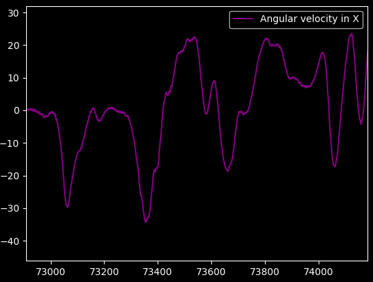
I've started out by loading some field-recorded gyroscope X data (pitch, "head bob") into an array, and plotting it:

Let's also plot the "desired output", which is basically the sum of the next 20 samples (which is 45ms at the 444Hz sample rate the glasses give me):

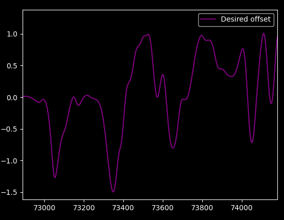
Nice, the noise went away.

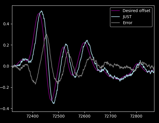
To "predict" the future orientation, the current code sums up the last 20 samples, to average out the noise, and add that to the current orientation. With constant angular velocity, this works great, but I never actually measured error or plotted it.

Let's plot it!

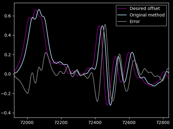
Ouch! That explains a lot, actually. That quarter wavelength phase change really hurts us, it introduces a lot of unnecessary error. In real life the picture looks like it hangs from a rubber band, and you can actually make it oscillate with your head. Very disorienting.

FIR filters to the rescue

The basic solution to all digital signal processing problem is FIR (finite impulse response) filters, which is a fancy way of saying convolution with a fixed length array, which is a fancy way of saying "sum up some past and future neighbors with specific weights".

In our case we only want past neighbors, since we don't have the future ones (i.e. we want a causal FIR filter).

The code is incredibly simple:

 1
 2
 3
 4
 5
 6
 7
 8
 9
10
11
12

def fir(indata, weights):
    result = []
    for i in range(len(desired_out)):
        if i < len(weights):
            result.append(indata[i])
        else:
            result.append(sum(
                indata[i-offset] * multiplier
                for offset, multiplier
                in enumerate(weights)
            ))
    return result

Now with this, we can go play with various filters. For example, our current filter looks like this: [0.05, 0.05, 0.05, ... times 20]

A much simpler one is "Just use the last sample": [1]

Huh. Maybe averaging wasn't such a good idea, because this is already way better.

A nice thing about FIRs (and convolutions in general) is that they are easy to combine.

For example, getting just the last sample is [1, 0], getting its older sibling is [0,1]. The average of the two is [0.5, 0.5].

The slope at a specific sample looks like this: [1,-1]. You can also average slopes, e.g. the average of [1,-1,0] and [0,1,-1] is [0.5, 0, -0.5] which is actually the slope between the last and the third to last points.

The use for this is to implement simple linear extrapolation: just add the last sample's slope to the last sample: [1, 0] + [1, -1] = [2, -1]

Of course it's not enough to add the slope once, we are predicting 20 samples ahead. Also we need to predict the sum of samples, so keep that in mind too (area under the slope is a triangle).

Long story short, I ended up with this linear extrapolation filter:

[70.0, 50.0, -50.0, -50.0]

Plotted, it looks like this:

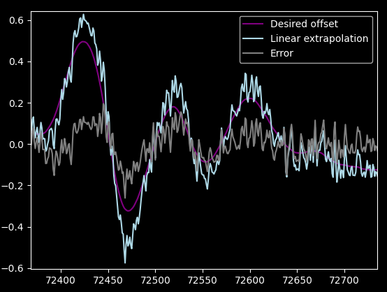
Note that the y scale is in degrees, and a 0.1° error is around 5 pixels on the glasses' screen.

Gradient descent

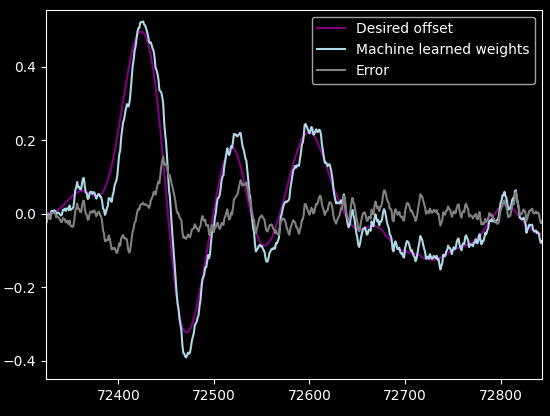
We are already doing pretty good, but instead of manually trying out ideas, why not let the computer work? That's right, we are going to do machine learning.

Well, not really, it's just simple gradient descent, but some years ago anything with a gradient descent or any Bayesian algorithm was called machine learning.

Oh by the way, there are more exact formulas with matrices to do this, but I failed Signal Processing I., and did good in AI-related classes instead. I have some big hammers in a worlds of nails.

Another reason is that GD is super easy: you just initialize a 30 element weight array with zeroes, and compute the gradient numerically:

 1
 2
 3
 4
 5
 6
 7
 8
 9
10

gradient = []
for i in range(len(weights)):
    weights = previous_weights.copy()
    weights[i] += 0.001
    gradient.append(
        previous_error - 
        # Sum of squared errors
        # over the whole dataset
        error(weights)
    )

To get a better estimate, add the gradient to the weights with some multiplier. Rinse and repeat, do 100000 steps and you get to a pretty good solution. Hope you used at least pypy or else you will sit there for some time.

There are a lot of implementations in python to do this (e.g. in scipy.optimize), and there's also one for Rust), but doing it manually was more fun.

Here's the result:

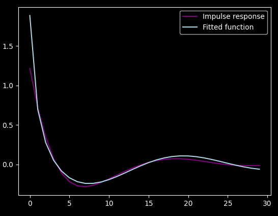
This is the impulse response:

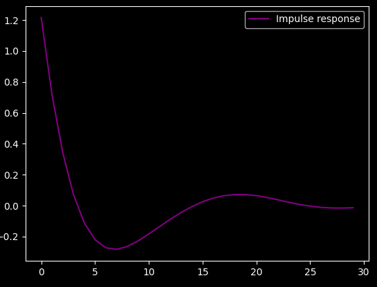
Huh. Looks like some kind of low-pass filter. I tried to fit sin(x*a+b)/(x*c+d) on it (with gradient descent :) ), but it didn't fit very well:

This was already late at night. I went to sleep.

Actual least squares

When I woke up, I decided to look at the closed form least squares algorithms anyway. I quickly realized that it is implemented in both Python and Rust.

Oh, and I rewrote the code to numpy, which made it 5x shorter and 100x faster. Also something I should've done from the beginning. Live and learn, I guess.

Now with that out of the way, I could compute the optimal weights for the FIR filter in milliseconds with np.linalg.lstsq().

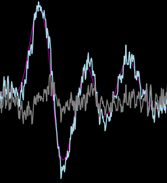
Comparing the Gradient Descent's impulse response solution to the actual Ordinary Least Squares (in light blue):

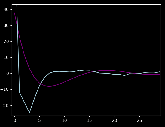
Hmm, it's not even close. But it does explain what I saw during "training": the first sample was going up and up, and the algorithm tried to adjust the rest of the weights according to that. It was very slow, it's a narrow hill in the error space.

As a bonus, it looks like I only need around 15 lookback samples.

I also tried out a different error metric, Least Absolute Deviation, and used scipy.optimize.minimize() this time to find a solution. It was only a tiny bit better (in the noise dampening department) than the least squares solution, but quite slower to calculate. So I decided against it.

Conclusion

Now I have a very fast weight calculator that can train to relatively large test datasets. I tried using only a super simple linear extrapolation, because it looked "good enough". Well, not really. That noise you saw in the earlier graphs was the resonance of the car when it's running. Looks like the glass doesn't use the built-in low-pass filter of the IMU and the engine resonance gets through. Extrapolated, it is actually pretty annoying, so I do have to use the "optimal" FIR to minimize this vibration of the screen while also predicting far enough ahead.

In the end, I just implemented a configurable FIR into our AR framework, and derive the weights offline from hundreds of megabytes of recordings.

Side note: blog driven development

Blogging while developing is the ultimate form of rubber ducking. I'm trying to explain what I'm doing to an unseen audience, which forces me to think a bit more slowly. It actually made development easier in the long run, and I caught 2-3 big errors on re-reading before publishing.

If you never tried, I can highly recommend doing it once.

If you need Augmented Reality problem solving, or want help implementing an AR or VR idea, drop us a mail at info@voidcomputing.hu