IMU prediction 2: Double Exponential Boogaloo

The whole FIR thing has served us well for the last few months, but some new developments has forced us to look into alternative prediction algorithms. Thankfully (?) I'm on many Discord channels, and someone mentioned Double Exponential Smoothing on one of them. Everyone loves a good clickbait, so you won't believe what happened in the end...

Prologue

As soon as I saw the first results from the exponential smoother test script (a modified version of the one I used for the FIR), I also started writing this blogpost. As I'm typing this, I have no idea whether it's actually going to work or not. So this is going to feel more like a journal than a technical description. Now that I think about it, most of my blogposts feel like this...

Anyway, let's go on another journey into the magical world of signal filtering.

Problem

When designing the IMU prediction algorithm for the AR glasses (to "know" where the user's head will be when the picture is actually displayed), we had some core assumptions:

1. The IMU signals arrive with a constant frequency
2. This frequency is the same, or at least similar across manufacturers
3. The delay between IMU signals and displaying pictures (the prediction interval) is constant

Turns out, none of this is true on Android. We have packet losses, variable frequencies, and worst of all, a lot of jitter in the IMU => display delay. The current prediction method just doesn't cut it anymore.

Recap: FIRs

Finite impulse response filter is a filter that gives a finite response to an impulse :)

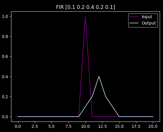
In the example above you see the impulse in purple, and the finite response (in this case, a delayed, smoothed signal) in light blue.

For this whole project, we will use "causal" filters, i.e. the filter can only "work with" past data. Also, it's "discrete", i.e. it works with discrete data points, as opposed to continuous (and hopefully smooth) functions. This way we can use simple sums instead of actual integrals.

We will not use scary math symbols today, only python. Our simple FIR filters will look like this for a single sample:

output[i] = sum(
    input[i-f] * impluse_response[f]
    for f in range(len(impulse_response))
)

Another way to look at it is that the FIR takes the whole input, delays and scales it with various amounts, and then sums up the components. For example, running the previous filter on a step function sums up the gray components:

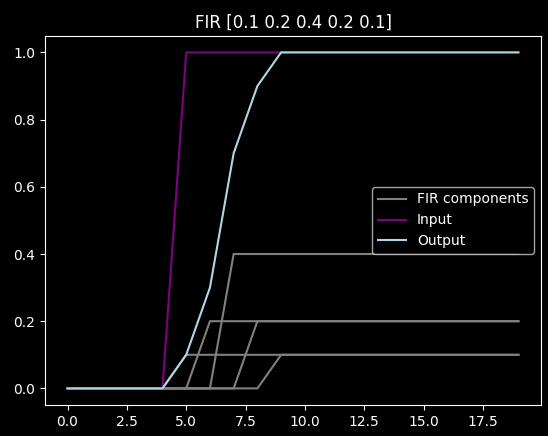
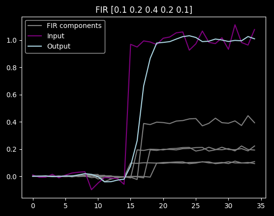
As you can see it delays and smooths out the step, which you may or may not want. It does smooth out noise too though:

Prediction

By default, a FIR will always delay the signal, so delays are easy to make:

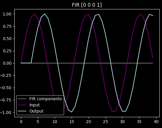
Prediction on the other hand is hard. Fortunately, in case of the sin function, if we want to predict it by e.g. a quarter wavelength, we can just derive it (and turn it into cos()). "Derivation" in discrete signal land is just subtracting the previous value from the current one, and applying the correct scaling:

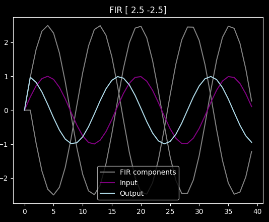
As you can see now the light blue leads by some 4-5 samples.

For more general signals, "deriving" gives you a slope, and you can use it to linearly extrapolate from the current data point. Or you can even calculate second or higher order derivatives and use those to have a polynomial extrapolation, and all of that can be done by just setting some values in the FIR array correctly.

Problems

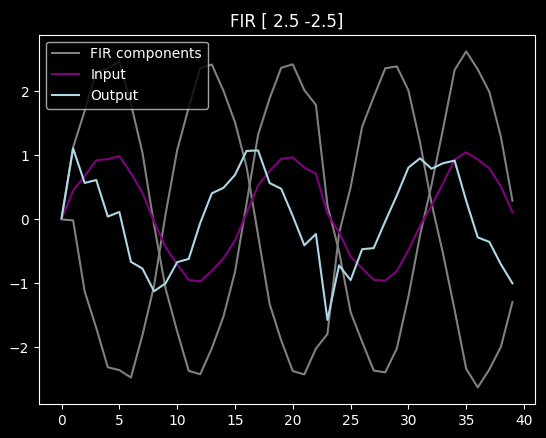
We have (at least) two problems with predicting with FIRs. First, they are very susceptible to noise (unless it includes some smoothing in the filter itself):

Second, we optimize FIRs for a specific prediction time. For example if we are predicting a linear function, the correct FIR array is a sum of two "sub" FIRs:

1. [1, 0]: Just the current sample
2. [1, -1] * prediction_period: Calculating the slope and using it to extrapolate

Yielding [1 + prediction_period, -prediction_period]. With higher order extrapolation, you would see higher powers of the prediction period in there too. With automatically optimized FIRs, we have no idea about the underlying polynomials, just the end result for a specific prediction period.

So the assumption was that for multiple prediction periods, we would need to train multiple FIRs, which sounded like an error-prone and potentially overfitted way to do things.

Exponential Smoothing

Simple exponential smoothing is an infinite impulse response causal filter. It is "recursively defined", i.e. the output value is defined using the previous output value (as opposed to the FIR, where the output only depends on the input and filter parameters).

The code is simple:

output = alpha * input + (1-alpha) * output

alpha is the "smoothing factor": 1 means no smoothing, close 0 means a lot of smoothing.

It can be approximated with the following FIR:

alpha * [1, (1-alpha), (1-alpha)^2, (1-alpha)^3 ...]

Some example outputs of the filter (clickable image):

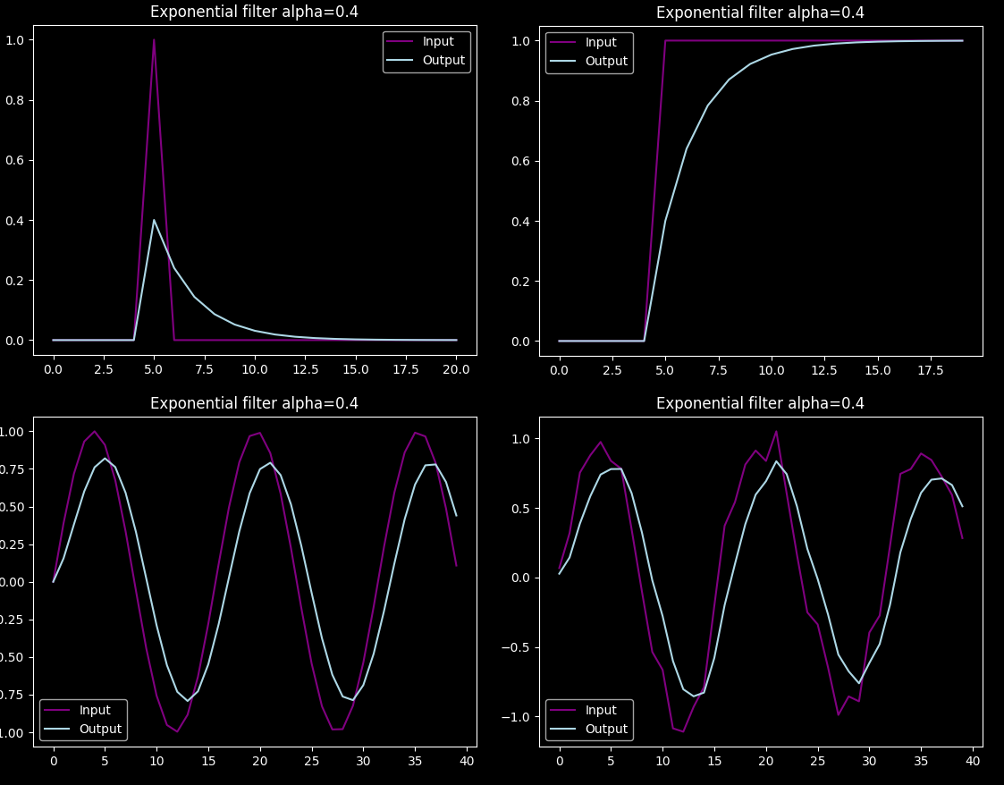
The bottom two are important: while exponential filtering gets rid of a lot of the noise, it does delay and dampen the signal.

Double Exponential Smoothing

To solve the above problem, people came up with Double Exponential Smoothing. It was developed to predict sales, but nowadays it's used to also predict stock prices, and it's very popular especially with the crypto technical analysis "gurus". That is pretty pseudo-scientific of course, but the method itself can be used for simpler problems where the signal has a slowly changing trend with some normal noise on it.

Like our head-movement prediction.

The trick of double exponential smoothing is that we not only calculate the "current" value, but also a trend (the first derivative). It is smoothed too, of course, with a parameter called beta.

The code looks like this:

previous_output = output
output = alpha * input + (1-alpha) * (input + trend)
trend = beta * (output - previous_output) + (1-beta) * trend

So we smooth between the actual output and a linearly extrapolated one, and then calculate the first derivative and smooth it into our trend approximation.

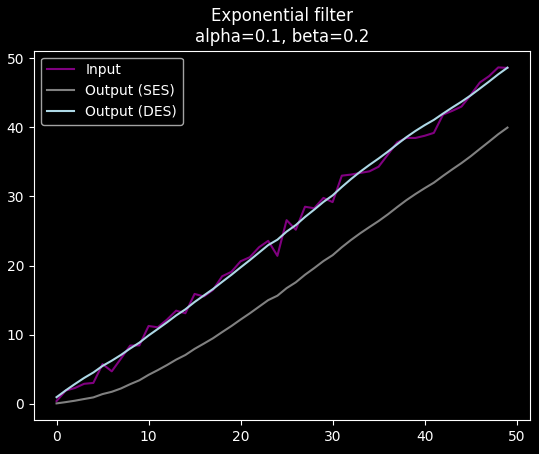
This has some nice properties, like being able to correctly follow a linear trend:

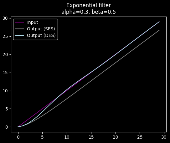
While also smoothing out noise:

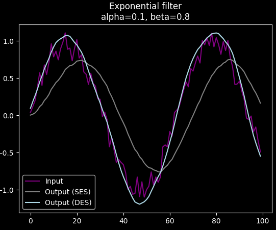
It can even filter out high frequency noise from a sin function without much additional delay:

Application to IMU filtering

The nicest property (for us at least) of DES is that it doesn't just give us a single prediction: it gives us a smoothed "current" value, but also a smoothed linear trend. With the linear trend, it's super easy to extrapolate an arbitrary amount into the future, you just do

prediction = output + trend * period

This of course only works for functions that are approximately (locally?) linear. Fortunately IMU stuff is in fact linear if you look at some 10 millisecond windows.

Some small thing though: the IMU readings are angular velocities, changes in these reading is angular acceleration (?). Remember, output is a velocity-like value, trend is an acceleration-like value, and we want a position-like value, so we have to integrate the prediction function:

predicted_angle = output * period + trend * period ** 2 / 2

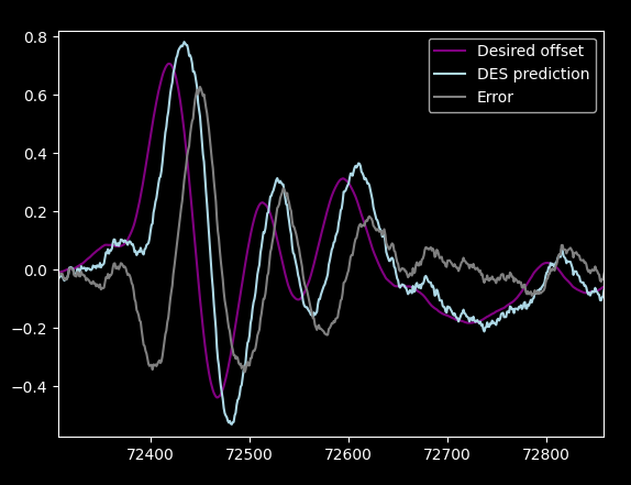
Anyway, here's a result with alpha and beta values optimized for our dataset (10 sample prediction):

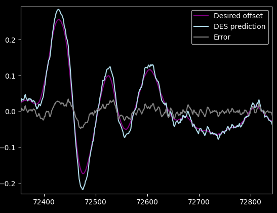
It does overshoot apparently, but there is not much noise, and it tightly hugs slopes. Cool. Even cooler is that it only has two relatively intuitive parameters, instead of 10+ opaque numbers.

Pretty charts and parameter sensitivity

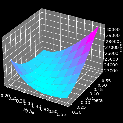
I've noticed while running optimization that the sum error over the dataset barely changes with the parameter values once they are in the correct range. This made me curious enough to make the best looking chart compilation of my life:

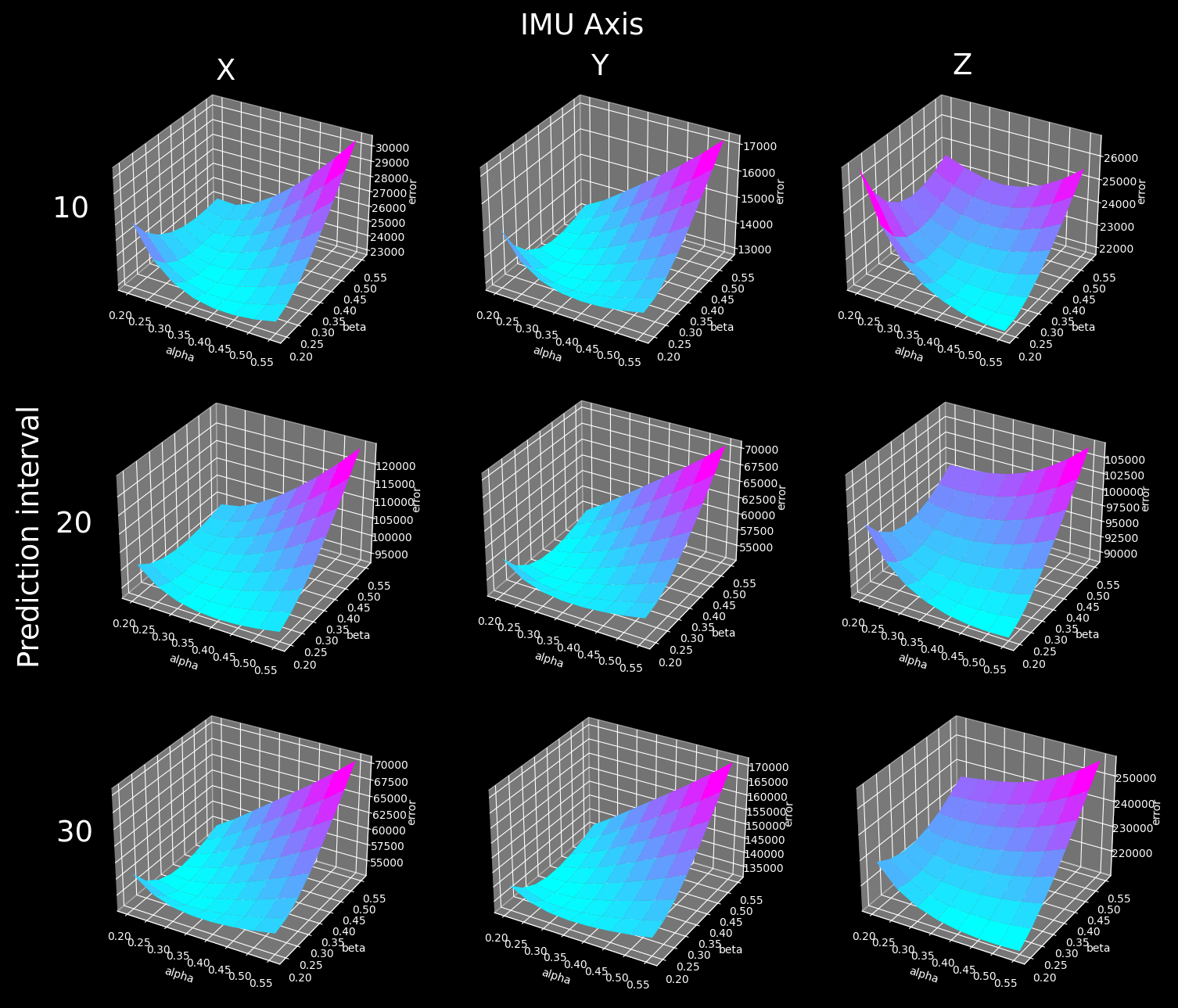
The image is clickable again, because while our website layout is super cool, it will never be good for displaying large images. Also it's not really mobile friendly. Maybe some day.

... anyway, it looks like the DES filter is not very sensitive to the actual parameter setting. We can be within 5-10% of the optimal error value with a single fixed parameter set. Or at most one parameter set per axis.

BTW, Axis X is looking up/down, Y is looking left/right, and Z is:

This explains why the Z sensitivity diagram looks so different: there's not much head tilt in the dataset (people rarely do that), and all the filter has to do is remove noise from an almost constant zero value.

Variants

This all was the basic DES filter. Unfortunately, the filtered output overshoots and delays quite a bit when predicting longer periods (30 in pic):

So I implemented some variants, to see if those help.

Higher order

The basic idea of DES is calculating a trend value. But what if we also approximated a trend of trend? Like an acceleration. I would call it Triple Exponential Filter, but unfortunately that's refers to a different adjustment about seasonality or something. Also not to be confused with Triple DES , a deprecated but surprisingly strong variant of DES (the encryption).

So if DES looks like this:

previous_output = output
output = alpha * input + (1-alpha) * (input + trend)
trend = beta * (output - previous_output) + (1-beta) * trend

Our higher order smoother could look like this:

previous_output = output
previous_trend = trend
output = alpha * input + (1-alpha) * (input + trend + trend2)
trend = beta * (output - previous_output) + (1-beta) * (trend + trend2)
trend2 = gamma * (trend - previous_trend) + (1-gamma) * trend2

And the prediction is:

predicted_angle =
    output * period +
    trend * period ** 2 / 2 + 
    trend2 * period ** 3 / 3

I put this third parameter into the optimizer, and it always came out with 0 as the "optimal value", i.e. the optimizer turned off the feature. So in this form it doesn't help. I think I derived it wrong, but I don't know what the correct derivation would be. Please tell me if you do.

Using input directly for trend

I also tried predicting the trend directly from the input as opposed to the pre-smoothed input:

output = alpha * input + (1-alpha) * (input + trend)
trend = beta * (input - previous_input) + (1-beta) * trend
previous_input = input

It made things worse. Like 20% more absolute error worse.

Damping on trend

To prevent overshooting for large trend values, I introduced a constant damping factor on the trend:

previous_output = output
output = alpha * input + (1-alpha) * (input + trend)
trend = beta * (output - previous_output) + (1-beta) * trend
trend *= damping

With damping being an optimizable parameter. The optimizer actually used it this time, and it did halve the overshoot amounts, at the cost of accuracy and, frankly, more complexity.

I didn't really go down this path, because ...

Compared to FIR

... I compared it to the optimized FIR outputs:

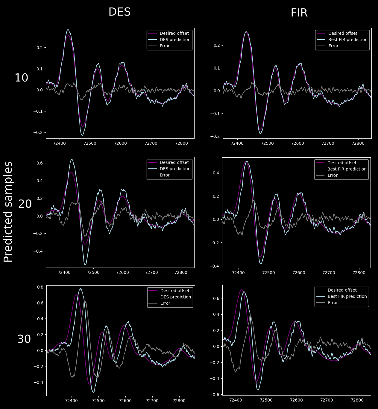
Oh my God it's so much worse. Keep in mind that both FIR and DES parameters were individually optimized for the dataset and the prediction period.

I was prepared for it being worse, because I saw that the absolute error of the DES was some 10% higher during optimization, and I was OK with that, because I like the simplicity of it, but this was pretty much unacceptable.

So I went back to experimenting with FIRs. (Yay, journal-like articles!)

FIR sensitivity to prediction range

So it turned out that it is assumption-challenging week, so I revisited the assumption that optimized FIR values "encode" high order polynomials of the prediction interval, so that we cannot just "scale" the FIR output and have a correct prediction.

The reason I had this hunch was that the optimized values behaved somewhat funky. For example if I increased the number of lookback samples, the impulse responses changed dramatically:

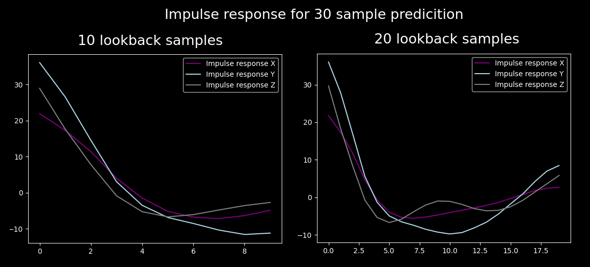
Just to test my assumption, I optimized several filters with various lookahead periods and looked at the optimized impulse responses:

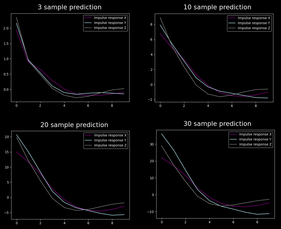
Apart from the unrealistically short one, they actually look similar. In fact, it looks pretty linear to the prediction interval (as explained above why).

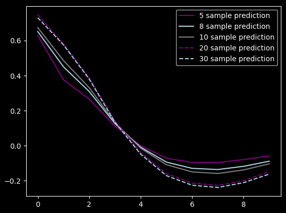
So I made this comparison chart where I scaled the various optimized curves:

]({attach}impulse_sensitivity.png)

Yeah, it's basically the same. I also visually confirmed it by using a filter optimized for 10 samples for predicting 30 samples just by multiplying it with 3. I'll show you the results, but before that, I tried to...

FIR variants

... have more parameters! We're already at 10, what's 10 more? What I did specifically is optimize one "universal" filter for a large range of prediction intervals, with the following model:

impulse_response = 
    const_response * lookahead_period +
    adjust_response * lookahead_period * lookahead_period / 2
output[i] = sum(
    input[i-f] * impluse_response[f]
    for f in range(len(impulse_response))
)

So basically I assumed that all impulse response parameters are linear to the lookahead period, and there are no higher order polynomials in there. Or to word it differently, I wanted to encode all the different curves of the previous pic with only two parameters per FIR sample. There is an integration in there too.

Here are the "universal weights" I got:

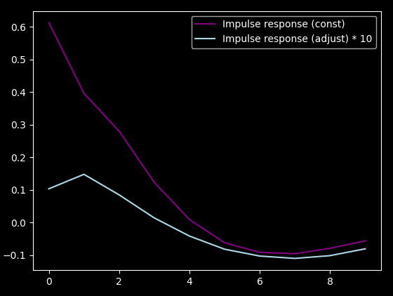
As you can see, the adjust_response part is barely "used", it's two orders of magnitude smaller than the const part, so it's still an order of magnitude smaller when using 10 sample lookahead. Thus, this filter does not do much better than a simple scaled one (for 30 sample prediction):

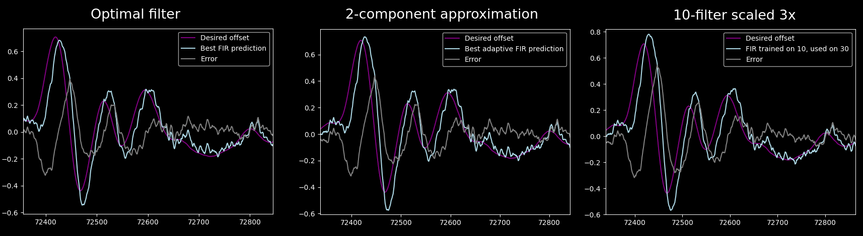
There are some differences in overshooting and delay, but not enough to warrant dealing with complexity. In fact, the peak absolute error barely changes.

Chosen solution

DES had a good run, but it fell a bit short, so I went with simply scaling the 10 sample filter.

Maybe the crypto bros and HFT alpha-farmers should look into using tuned FIRs instead of exponential stuff, it would probably work much better. Or maybe not.

If you need Augmented Reality problem solving, or want help implementing an AR or VR idea, drop us a mail at info@voidcomputing.hu